
Conditional formatting is a feature in various spreadsheet applications that permits you to apply specific formatting to cells that meet certain criteria or specified condition. It is mostly used as a color-based formatting to highlight, emphasize or differentiate among statistics and information stored in a spreadsheet.
Conditional formatting makes it easy to highlight interesting cells (ranges of cells), highlight unusual values, and visualize data by using data bars, color scales, and icon sets that correspond to particular differences within the data.
Benefits of using Conditional Formatting
- It is one of the simplest yet powerful feature in Excel Spreadsheets.
- It gives you the ability to quickly add a visual analysis layer over your data set. It permits you to visually analyze your data, based on a large number of condition types,
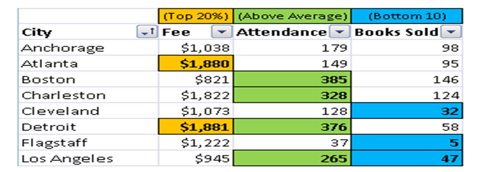
- Greater than, Less than, Between
- Above / Below Average
- Top / Bottom 10
- Top / Bottom 10%
- Duplicates / Unique
- Dates – Dynamic or a fix date range
- Text containing
- You are able to create heat maps, show increasing/decreasing icons, Harvey bubbles, and a lot more using conditional formatting in Excel.
- The spreadsheet will also have the ability to format itself as you are working on it in real time.
- Helps in answering questions which are important for taking decisions.
- Helps in understanding distribution and variation of critical data.
There are 5 types of conditional formatting visualizations
Conditional formatting is a feature in various spreadsheet applications that permits:
- Background Color Shading (of cells)
- Foreground Color Shading (of fonts)
- Data Bars.
- Icons (4 different image types)
- Values.
Using conditional formatting in Excel
To apply conditional formatting to an Excel workbook, follow the below steps.
- Open or create an Excel workbook.
- Then select the range of cells you desire. Entire workbook can also be selected using Ctrl+A.
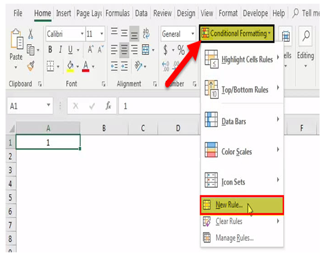
- On the Home tab, select the Conditional Formatting option, then select the sub option New Rule.
- In the New Formatting Rule window, under Select a Rule Type choose the type of rule you want to create.
- Under the heading Edit the Rule Description, select the desired Format Style, and select or enter the required criteria for the Rule Type and Format Style selected.
- Finally, Click OK to save and apply the rule to the selected cells.
Using Excel conditional formatting with formula.
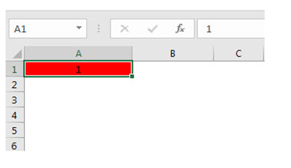
The aim is to highlight the Cell A1 with red color if the value in A1 cell will be
- Open an Excel workbook.
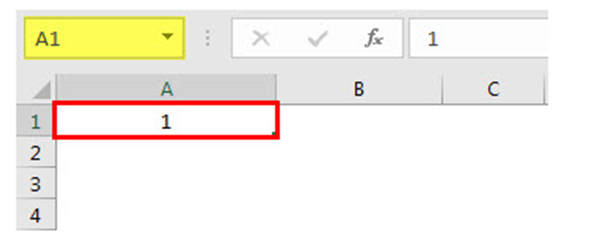
- Then, Select any cell A1
3. Click Conditional Formatting in Excel Styles group, and then click New Rule
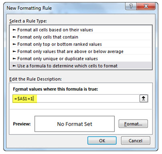
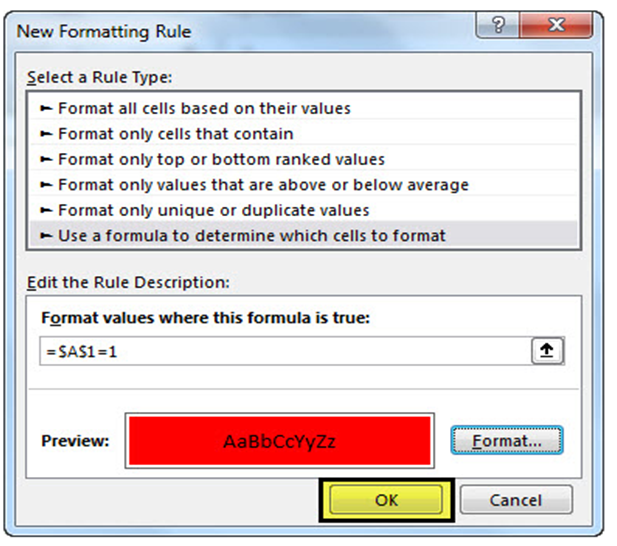
4.Click the last rule, Use a formula to determine which cells to format under Select a Rule Type.
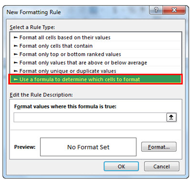
5.Click inside the Format values where this formula is true. Then, choose the cell that you want to use for the conditional formatting in excel.

6. Modify the value in step 6 to be =$A$1=1
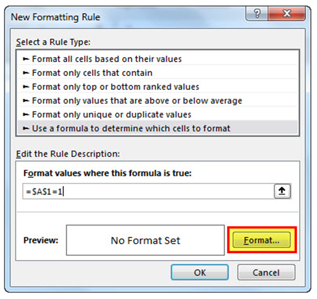
7. Click Format
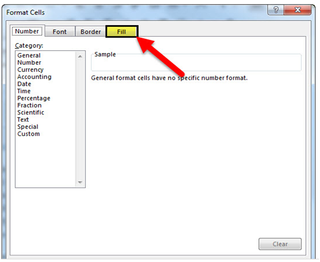
8. In the Format Cells dialogue box, click the Fill.
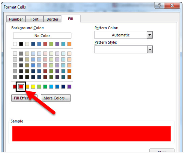
9. Click the color “red,” and then click OK
10. In the New Formatting Rule dialogue box, click OK
11. In cell A1, type 1, and then press the ENTER key
Using conditional formatting will help you visually explore and analyze data, detect critical issues, and identify patterns and current trends.
Also read about: Vlookup