

What exactly is VLOOKUP in excel?
VLOOKUP in excel stands for ‘Vertical Lookup’. The VLOOKUP function in Excel is a tool to scan a certain piece of information in a table or data set and extracting some corresponding data/information. For example, suppose you have a list of products with their prices, you can search for the price of a particular item.
VLOOKUP is an Excel function to present data in a table organized vertically. VLOOKUP supports both approximate and exact matching. Basically, VLOOKUP allows you to search for required specific information in your spreadsheet.
The VLOOKUP function in Excel execute a case-insensitive lookup.
VLOOKUP Formula
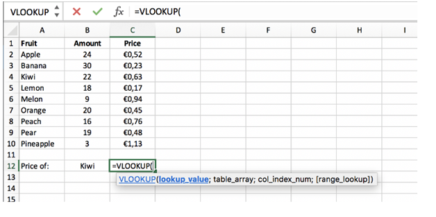
=VLOOKUP(lookup_value, table_array, col_index_num, [range_lookup])
How to use VLOOKUP in Excel
Step 1: Organize the data
Step one for effectively using the VLOOKUP function is to ensure your data is well organized and suitable for using the function.
VLOOKUP always looks for the new data from left to right direction of your current data., so make sure that the data you want to look up is to the left side of the sheet in correspondence with the data you want to draw out.
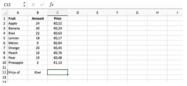
In the below example we have a list of fruits, the amount in stock and the current price. We want to find out the price of kiwi’s in this table.
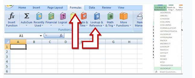
Note: You can find the VLOOKUP function under the “Formulas tab” _”Lookup & Reference”_”VLOOKUP”
Step 2: Tell the function what value to look for
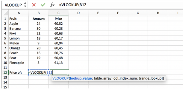
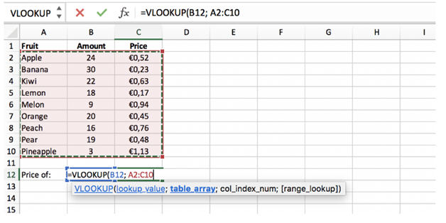
In this step, we brief Excel what to search for (lookup value) We start by typing the formula “=VLOOKUP(“ and then choose the cell that contains the information we want to lookup for.
Step 3: Tell the function the range to look for
The next step is to select the table where the data is located in the spreadsheet, and brief Excel to scan in the left most column for the information we selected in the previous step.
In this case the ‘Kiwi’ is in cell B12:
In this case it is range (A2:C10):
Step 4: Tell Excel which column to output the data from
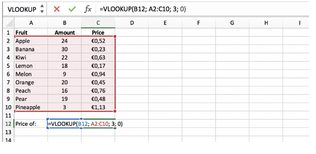
In step 4, we need to brief Excel as to which column contains the data that we want to have as an output from the VLOOKUP function. For this, Excel needs a number that matches to the column number within the table.
In this example it is column 3, followed by ‘;’ and ‘0’ or ‘FALSE to get an exact match with the lookup value of ‘Kiwi’:
Step 5: Exact or approximate match
This final step is to inform Excel if you’re seeking out an exact or approximate match by entering “True” or “False” in the formula.
In our VLOOKUP if we want an exact match we will type “FALSE” in the formula. We would get an approximate match, if we use “TRUE” as a parameter.
An approximate match would be useful when we look for an exact figure that might not be contained in the table, This will unable you to prevent errors in the VLOOKUP formula.
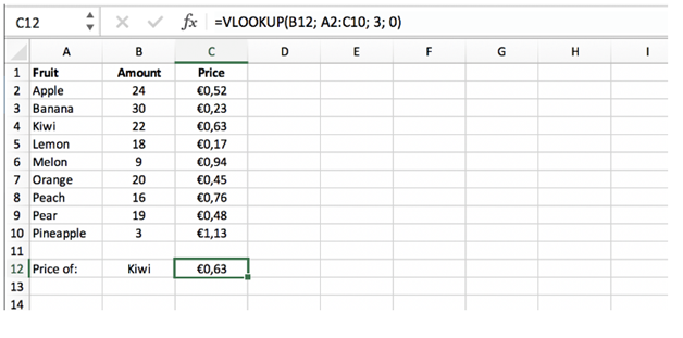
Once we press enter, we get the corresponding price from the row that contains the value of ‘Kiwi’ within the selected table array:
To use VLOOKUP the user only has to change a certain value in one worksheet and it will automatically be changed in all the other relevant places.