What exactly is HLOOKUP in excel?

HLOOKUP in Excel stands for ‘Horizontal Lookup’. The HLOOKUP function in excel makes the excel search for a certain value in a row also called as ‘table array, in order to return a value from a different row in the same column. HLOOKUP always searches for a value in the first row of a table/data. When a match is found, it retrieves a value at that column from the given row.

The function is used to retrieve information from a table by searching a row for the matching data and producing from the corresponding column. VLOOKUP searches for the value in a column, whereas HLOOKUP searches for the value in a row.

HLOOKUP Formula

HLOOKUP(lookup_value, table_array, row_index_num, [range lookup])

HLookup V/S VLOOKUP?

• HLOOKUP and VLOOKUP are the two functions in Microsoft Excel that allows you to use a section of your spreadsheet as a lookup table.

• Use HLOOKUP while lookup values are positioned inside the first row of a desk. Use VLOOKUP when research values are placed in the first column of a desk

• HLOOKUP is to lookup for a value horizontally in a table. The VLOOKUP function is used to look up a specified value in a table array organized vertically.

• HLookup looks for a particular value in the top row of a table and in return giving back the value in the same column.Whereas VLookup gives result from a specified column against that value in the same row but in the subsequent column.

What is Hlookup used for in Excel?

HLOOKUP in excel is used when the values to be compared are located in the top row of a table of data, and we want to look down a specified number of rows. The function conduct a rough match either in a one-row or one-column range and return a corresponding piece of data in another row or column.

How to use HLOOKUP in Excel

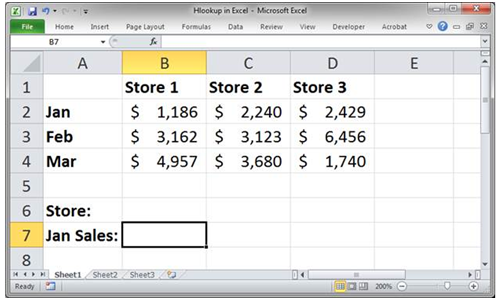
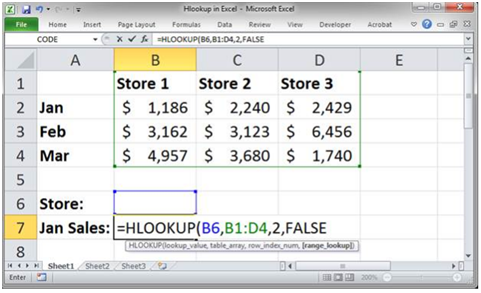
Let`s take the following table. Here, we have a basic sales at various stores and we want to get the January sales in cell B7.

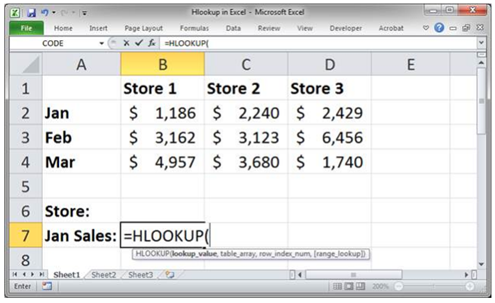
Type the function in the cell where you want the result to be displayed. We start by typing the formula “=HLOOKUP(“ and then choose the cell that contains the information we want to lookup for.

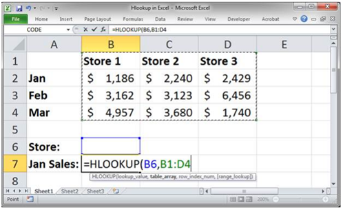
The next step is to select the table where the data is located in the spreadsheet, and brief Excel to scan the selected table for the information we selected in the previous step. We will reference a cell, B6.

Just be sure that the first row of the table array is the same row that you will use to search for the lookup_value.

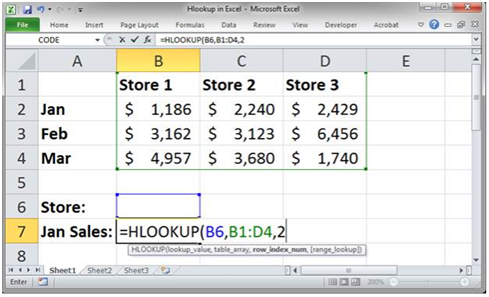
Now, tell the function from which row you want to return data (note: that the first row is the lookup row).  Since January sales are the second row from the top row of the table array, we insert no 2.

Finally, By entering “True” or “False” in the formula, we can inform the Excel if you’re seeking out an exact or approximate match.

In our HLOOKUP if we want an exact match we will type “FALSE” in the formula(exact match with the name of the store for the lookup_value). If we use “TRUE” as a parameter, we will get an approximate match.

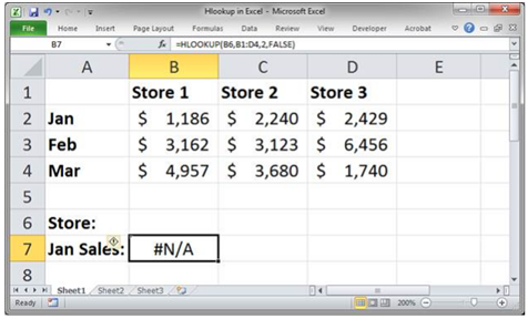
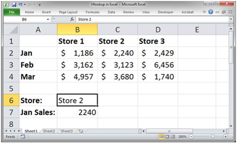
Finally, Type a store name, Hit enter and you are done to get the result!

Also, read our blog on How to use Concatenate